Introduction
Variational Autoencoders (VAEs) [Kingma & Welling, 2013] are powerful generative models that combine deep learning with variational inference. Unlike standard autoencoders, VAEs learn a probabilistic latent representation, enabling smooth interpolation, meaningful sampling, and principled uncertainty quantification.
What This Study Covers
This work presents three experiments exploring VAE behavior on the MNIST dataset:
- 2D Latent Space VAE: A baseline experiment with 2-dimensional latent space for easy visualization and interpretation
- 3D Latent Space Extension: Extending to 3 dimensions to examine trade-offs between interpretability and representational capacity
- Correlated Prior Distribution: Exploring non-isotropic priors using custom covariance matrices and Cholesky decomposition
Each experiment includes complete Jupyter notebooks with runnable code, mathematical derivations from first principles, and comprehensive visualizations. We discuss both what works and the limitations of these approaches.
About the Dataset
All experiments use MNIST (28×28 grayscale handwritten digits). This is a simple dataset ideal for understanding VAE concepts, but the findings may not generalize to complex, high-resolution images which would require different architectures and training procedures.
Theoretical Background
2.1 Variational Inference Framework
VAEs formalize generative modeling within a probabilistic framework. Given observed data \(x\), we aim to learn:
- Generative model: \(p_\theta(x, z) = p_\theta(x|z)p(z)\), where \(p(z)\) is a prior over latent variables and \(p_\theta(x|z)\) is the likelihood
- Approximate posterior: \(q_\phi(z|x)\) that approximates the intractable true posterior \(p_\theta(z|x)\)
The parameters \(\theta\) (decoder) and \(\phi\) (encoder) are jointly optimized to maximize the Evidence Lower Bound (ELBO), which lower-bounds the log-likelihood \(\log p_\theta(x)\).
2.2 Core Components
Encoder
Compresses input \(x\) into latent variables \(z\)
\(q(z|x) = \mathcal{N}(\mu, \sigma^2)\)
Latent Space
Probabilistic representation
\(p(z) = \mathcal{N}(0, I)\)
Decoder
Reconstructs from latent samples
\(p(x|z)\)
2.3 The Reparameterization Trick
A critical innovation in VAEs is the reparameterization trick, which enables backpropagation through stochastic sampling. Rather than sampling \(z \sim q_\phi(z|x)\) directly (which blocks gradients), we reparameterize:
By isolating the stochasticity in \(\epsilon\) (independent of \(\phi\)), gradients can flow through the deterministic transformations \(\mu_\phi\) and \(\sigma_\phi\). This is essential for end-to-end training via gradient descent.
2.4 Complete Loss Function Derivation
Objective: The VAE maximizes the ELBO, which is equivalent to minimizing:
Step 1: KL Divergence for Diagonal Gaussian Posterior
We need to compute \(D_{KL}(q_\phi(z|x) \| p(z))\) where:
- \(q_\phi(z|x) = \mathcal{N}(\mu, \text{diag}(\sigma^2))\) (approximate posterior)
- \(p(z) = \mathcal{N}(0, I)\) (prior)
Write out Gaussian PDFs:
Take expectation w.r.t. \(q_\phi(z|x)\):
- Term 1: \(\mathbb{E}[-\frac{1}{2}\sum_{i}\log(\sigma_i^2)] = -\frac{1}{2}\sum_{i}\log(\sigma_i^2)\)
- Term 2: \(\mathbb{E}[-\frac{1}{2}\sum_{i}\frac{(z_i-\mu_i)^2}{\sigma_i^2}] = -\frac{k}{2}\)
- Term 3: \(\mathbb{E}[\frac{1}{2}\sum_{i}z_i^2] = \frac{1}{2}\sum_{i}(\sigma_i^2 + \mu_i^2)\)
Final closed-form KL divergence:
Step 2: Reconstruction Loss
For Binary Data (MNIST):
Assume each pixel is independent Bernoulli:
Taking the log:
Therefore, reconstruction loss is binary cross-entropy:
For Continuous Data:
Assume Gaussian likelihood \(p_\theta(x|z) = \mathcal{N}(x; g_\theta(z), \sigma^2I)\):
Ignoring constants, this gives MSE:
Step 3: Complete VAE Loss
Final training objective (scaled negative ELBO):
In practice, we use per-pixel and per-latent-dimension averages of the negative ELBO. For a Gaussian likelihood (MSE reconstruction), ignoring constants, a convenient implementation is:
where:
- \(z = \mu_\phi(x) + \sigma_\phi(x) \odot \epsilon\) with \(\epsilon \sim \mathcal{N}(0, I)\)
- \(D\) = data dimensionality (784 for MNIST 28×28)
- \(d\) = latent dimensionality (2, 3, etc.)
For binary data (MNIST with Bernoulli likelihood):
Use binary cross-entropy instead of MSE:
Implementation Note
In code, we work with \(\log(\sigma^2)\) for numerical stability and compute the KL term as follows:
# Encoder outputs
z_mean = encoder_mean(x)
z_log_var = encoder_log_var(x)  # log(σ²) not σ²

# KL loss: sum over latent dimensions, then average over batch
kl_loss = -0.5 * tf.reduce_sum(1 + z_log_var - tf.square(z_mean) - tf.exp(z_log_var), axis=-1)

# Reparameterization
z = z_mean + tf.exp(0.5 * z_log_var) * epsilon  # σ = exp(0.5 * log(σ²))
This expression is exactly the closed-form KL divergence derived above, written in terms of \(\log(\sigma^2)\).
Reconstruction Term
Ensures output fidelity
Binary cross-entropy or MSE
KL Divergence Term
Regularizes latent space
Closed-form for Gaussians
Experiment 1: 2D Latent Space VAE
📓 Interactive Jupyter Notebook
Run this experiment yourself! The complete notebook includes all code, training loops, and visualizations.
Notebook: vae.ipynb
Open Notebook →Overview
This first experiment uses a 2-dimensional latent space to establish a baseline and enable direct visualization. The convolutional architecture consists of:
Encoder:
- Conv2D(32 filters, 3×3, stride=2, ReLU) → 14×14×32
- Conv2D(64 filters, 3×3, stride=2, ReLU) → 7×7×64
- Flatten → Dense(16, ReLU)
- Dense(2) for μ, Dense(2) for log σ²
Decoder:
- Dense(7×7×64, ReLU) → Reshape(7, 7, 64)
- Conv2DTranspose(64 filters, 3×3, stride=2, ReLU) → 14×14×64
- Conv2DTranspose(32 filters, 3×3, stride=2, ReLU) → 28×28×32
- Conv2DTranspose(1 filter, 3×3, sigmoid) → 28×28×1
Training Results
After 30 epochs of training on MNIST (70,000 images), the model achieved:
Note: These metrics are from the notebook training run. The non-zero KL divergence (~3.9) suggests the model is using the latent variables (no posterior collapse), while still staying reasonably close to the prior distribution.
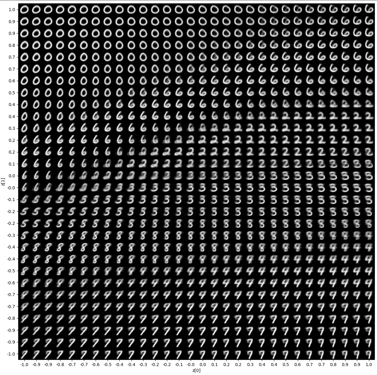
Visualization 1: Latent Manifold
By sampling a grid of points in the 2D latent space and decoding them, we can visualize the learned manifold:
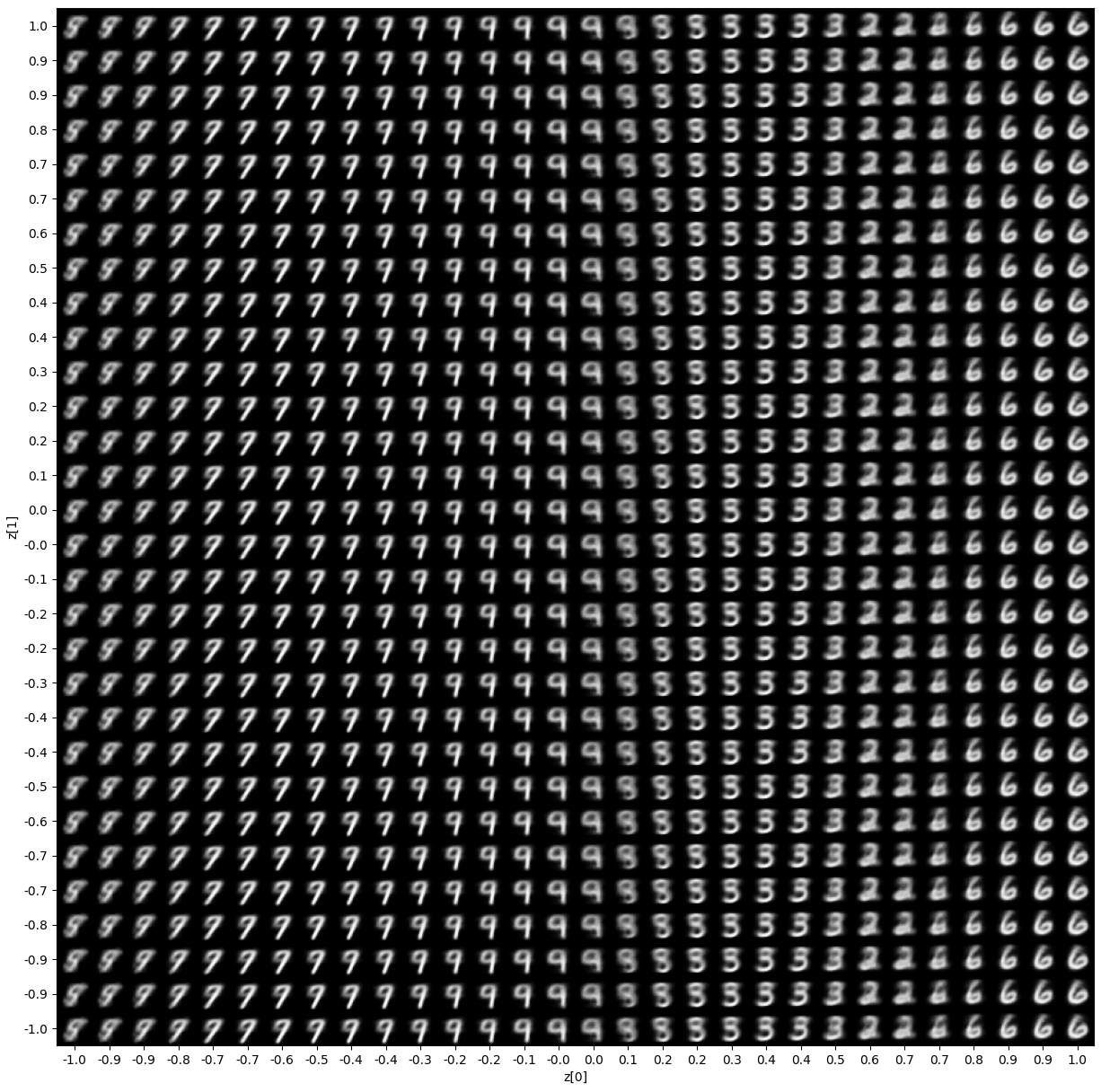
2D manifold of generated digits. Smooth transitions demonstrate the learned continuity of the latent space.
Key Observations
- Smooth transitions between different digit classes
- Continuous manifold structure without discontinuities
- Neighboring points produce visually similar digits
- Edge regions show interesting interpolations between classes
Visualization 2: Clustering
Plotting the latent encodings of test samples reveals natural clustering by digit class:
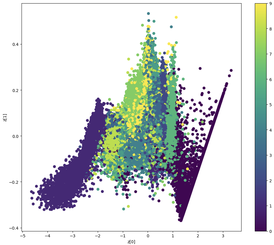
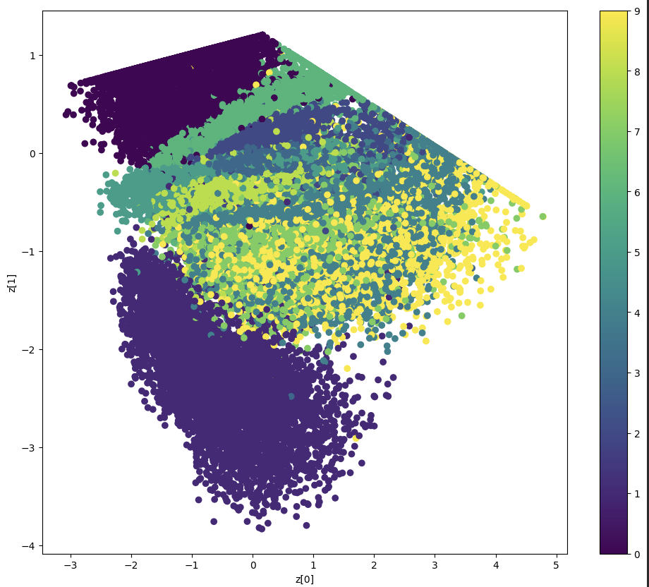
Distribution of digit classes in 2D latent space. Colors represent digit labels (0-9).
Key Observations
- Each digit class forms distinct clusters
- Similar digits (e.g., 3 and 8, 4 and 9) positioned near each other
- Some overlap indicates visual similarity
- Encoder learned meaningful semantic relationships
Experiment 2: 3D Latent Space Extension
📓 Interactive Jupyter Notebook
Explore the 3D latent space with interactive visualizations including 3D scatter plots and 2D projections.
Notebook: VAE3D.ipynb
Open Notebook →Motivation
While 2D latent spaces are easy to visualize, they may be too restrictive for complex data. By extending to 3D, we hypothesize we can:
- Increase representational capacity
- Capture more factors of variation in the data
- Achieve better reconstruction quality
- Potentially improve disentanglement between latent factors
The implementation is straightforward—we simply change the latent dimension from 2 to 3:
latent_dim = 3  # Changed from 2
# All other architecture remains the same
Training Results
After 30 epochs with the same hyperparameters as Experiment 1:
Key Finding: The 3D latent space achieved marginally lower total loss (~164 vs ~165), indicating slightly better reconstruction. The additional dimension provides more capacity to represent digit variations.
Visualization 1: 3D Scatter Plot
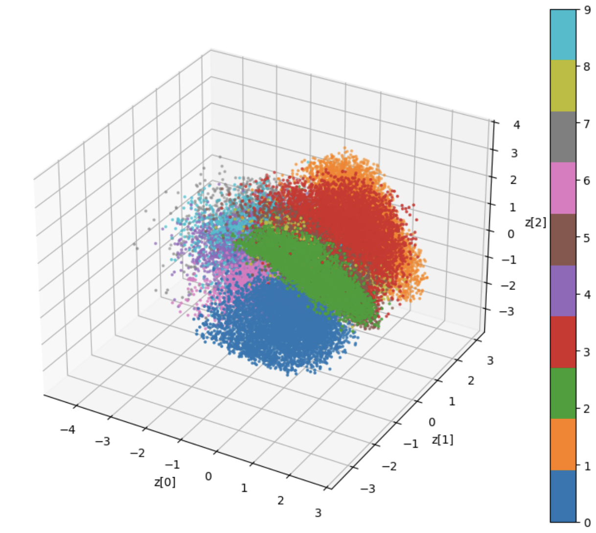
3D scatter plot of encoded MNIST digits. Clear clustering with enhanced separation.
Visualization 2: Pairwise 2D Projections
To understand information distribution across dimensions, we plot pairs (z₀, z₁), (z₁, z₂), and (z₀, z₂):
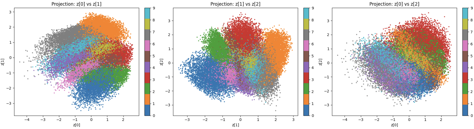
Pairwise 2D projections of 3D latent space. Each subplot shows one pair of latent dimensions.
Key Observations
- Each dimension contributes meaningful variation
- Clusters remain coherent across all projections
- No single dimension dominates
Visualization 3: 2D Cross-Sections
By fixing z₂ and varying (z₀, z₁), we can slice through the 3D manifold:
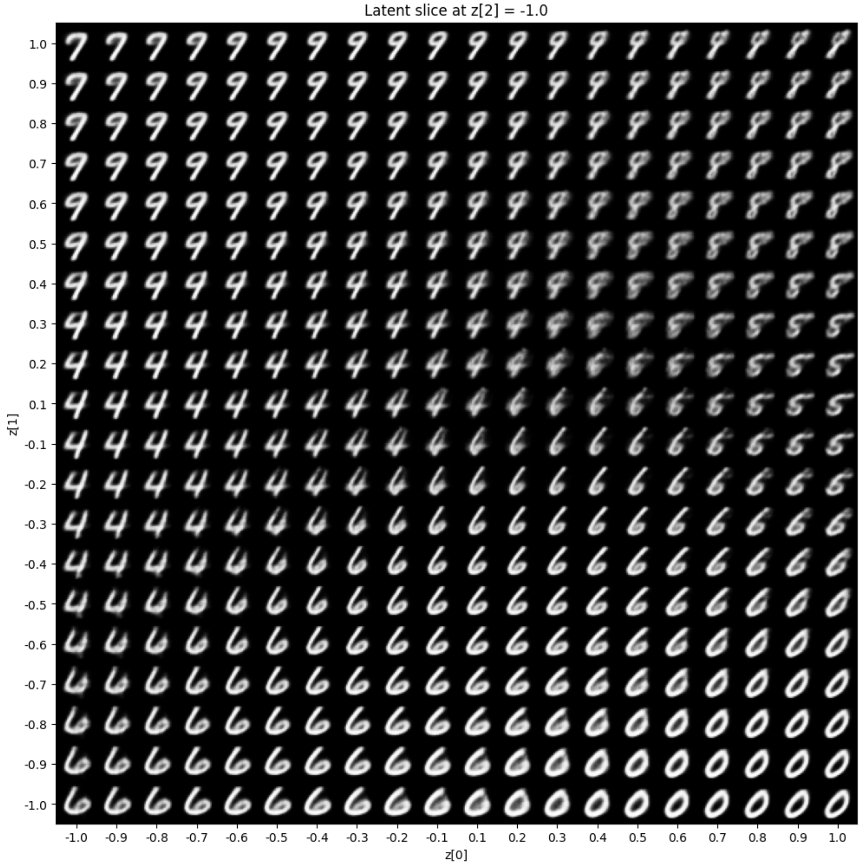
z₂ = -1.0
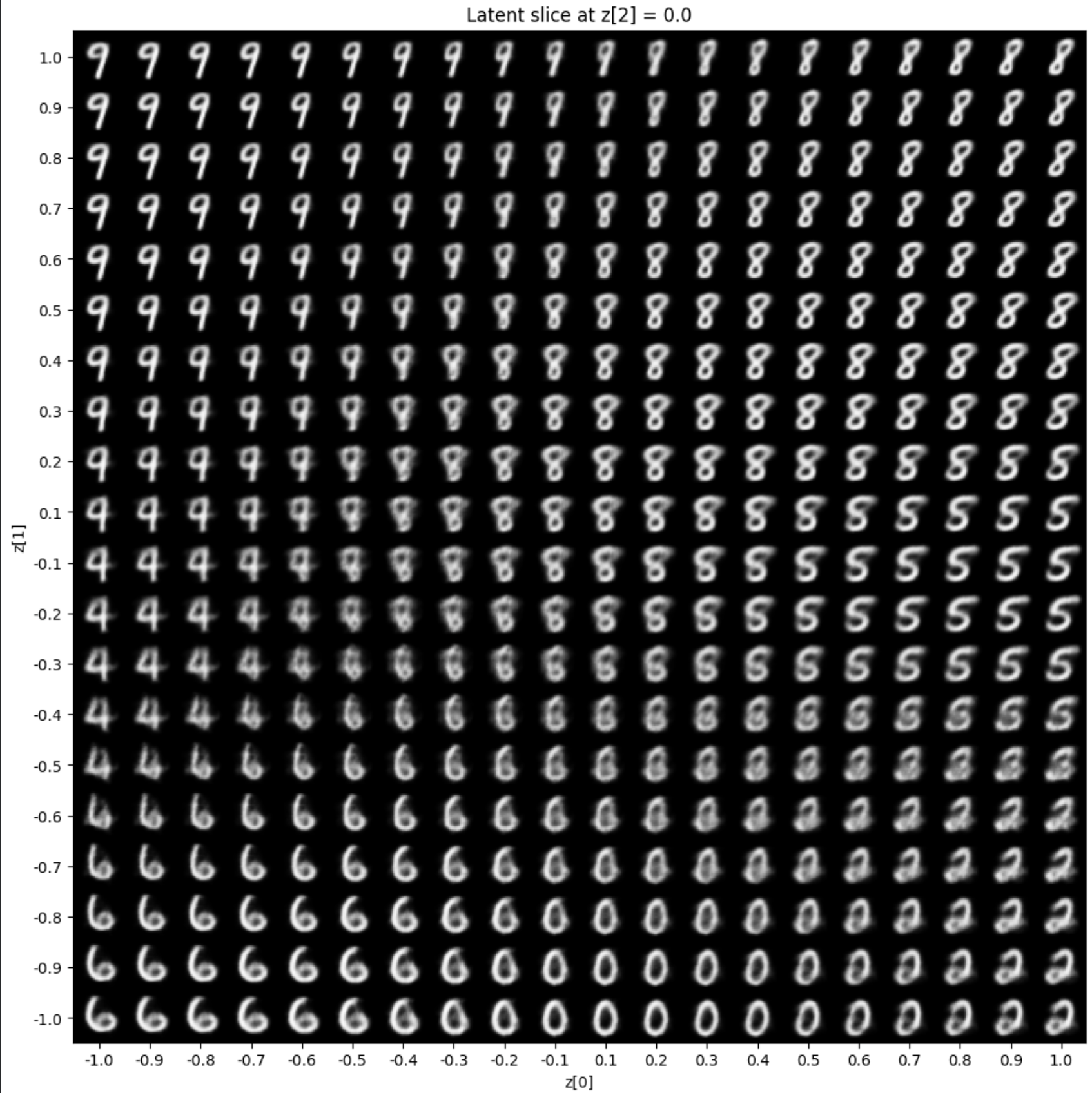
z₂ = 0.0
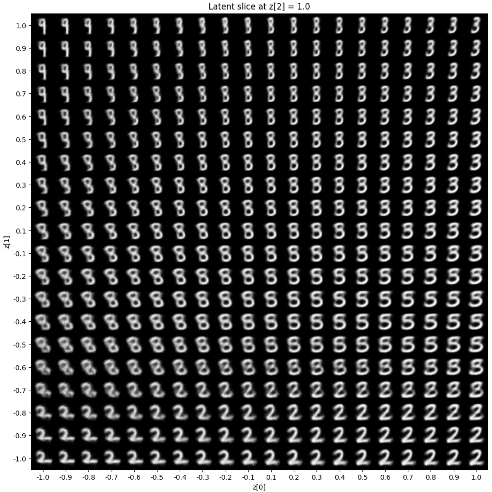
z₂ = 1.0
Key Observations
- Different slices show different digit styles
- z₂ primarily modulates stroke thickness and style
- z₀ and z₁ capture digit identity
- Smooth transitions demonstrate continuity
Experiment 3: Correlated Prior Distribution
📓 Interactive Jupyter Notebook
Implement a VAE with custom covariance matrix using Cholesky decomposition and custom KL divergence.
Notebook: VaeMat.ipynb
Open Notebook →Motivation
Experiments 1 and 2 used the standard isotropic prior:
This assumes independence between latent dimensions. However, real-world factors are often correlated (e.g., stroke thickness and digit style). In this experiment, we explore a correlated Gaussian prior:
where \(\Sigma\) is a full covariance matrix with off-diagonal elements.
Implementation Changes
1. Modified Sampling Layer
Replace standard reparameterization with Cholesky-based sampling:
# Standard: z = μ + σ ⊙ ε
# Correlated: z = μ + L ε, where Σ = L Lᵀ

L = np.linalg.cholesky(Sigma)
z = z_mean + tf.matmul(epsilon, L.T)
For this experiment, we use:
This introduces positive correlation between z₀ and z₁
2. Updated KL Divergence
The KL divergence must account for the correlated prior. This is the standard KL formula between two Gaussians where:
- \(q(z|x) = \mathcal{N}(\mu, \text{diag}(\sigma^2))\) — approximate posterior (diagonal covariance)
- \(p(z) = \mathcal{N}(0, \Sigma)\) — correlated prior (full covariance matrix)
Results
Generated manifold showing tilted digit transitions
Latent encodings (z₀, z₁) under correlated prior
Key Observations
- Manifold appears tilted and stretched
- Latent clusters form elongated, rotated patterns
- Geometry matches correlation structure in Σ
- Reconstruction quality remains similar to isotropic case
Limitations and Discussion
5.1 Reference Implementation
Note: For simplicity, the code below uses a fully-connected (dense) architecture. The main experiments in Sections 3–5 use the convolutional architectures described earlier.
import numpy as np
import tensorflow as tf
from tensorflow import keras
from tensorflow.keras import layers

# Hyperparameters
latent_dim = 2
input_shape = (28, 28, 1)

# Encoder
encoder_inputs = keras.Input(shape=input_shape)
x = layers.Flatten()(encoder_inputs)
x = layers.Dense(512, activation='relu')(x)
x = layers.Dense(256, activation='relu')(x)

z_mean = layers.Dense(latent_dim, name='z_mean')(x)
z_log_var = layers.Dense(latent_dim, name='z_log_var')(x)

# Sampling layer
def sampling(args):
    z_mean, z_log_var = args
    batch = tf.shape(z_mean)[0]
    dim = tf.shape(z_mean)[1]
    epsilon = tf.keras.backend.random_normal(shape=(batch, dim))
    return z_mean + tf.exp(0.5 * z_log_var) * epsilon

z = layers.Lambda(sampling, name='z')([z_mean, z_log_var])

encoder = keras.Model(encoder_inputs, [z_mean, z_log_var, z], name='encoder')

# Decoder
latent_inputs = keras.Input(shape=(latent_dim,))
x = layers.Dense(256, activation='relu')(latent_inputs)
x = layers.Dense(512, activation='relu')(x)
x = layers.Dense(28 * 28, activation='sigmoid')(x)
decoder_outputs = layers.Reshape((28, 28, 1))(x)

decoder = keras.Model(latent_inputs, decoder_outputs, name='decoder')

# VAE Model
class VAE(keras.Model):
    def __init__(self, encoder, decoder, **kwargs):
        super(VAE, self).__init__(**kwargs)
        self.encoder = encoder
        self.decoder = decoder

    def call(self, inputs):
        z_mean, z_log_var, z = self.encoder(inputs)
        reconstructed = self.decoder(z)

        # KL divergence loss
        kl_loss = -0.5 * tf.reduce_mean(
            z_log_var - tf.square(z_mean) - tf.exp(z_log_var) + 1
        )
        self.add_loss(kl_loss)

        return reconstructed

# Compile and train
vae = VAE(encoder, decoder)
vae.compile(optimizer='adam', loss='binary_crossentropy')

# Load MNIST data
(x_train, y_train), (x_test, y_test) = keras.datasets.mnist.load_data()
x_train = x_train.astype('float32') / 255.0
x_train = np.expand_dims(x_train, -1)
x_test = x_test.astype('float32') / 255.0
x_test = np.expand_dims(x_test, -1)

# Train
vae.fit(x_train, x_train, epochs=30, batch_size=128, validation_split=0.1)
Visualization Code
import matplotlib.pyplot as plt

# 1. Plot latent space clusters
z_mean, _, _ = encoder.predict(x_test)
plt.figure(figsize=(10, 8))
plt.scatter(z_mean[:, 0], z_mean[:, 1], c=y_test, cmap='tab10', alpha=0.5)
plt.colorbar()
plt.xlabel('z[0]')
plt.ylabel('z[1]')
plt.title('2D Latent Space Clustering')
plt.show()

# 2. Generate manifold grid
n = 20
grid_x = np.linspace(-3, 3, n)
grid_y = np.linspace(-3, 3, n)

figure = np.zeros((28 * n, 28 * n))
for i, yi in enumerate(grid_y):
    for j, xi in enumerate(grid_x):
        z_sample = np.array([[xi, yi]])
        x_decoded = decoder.predict(z_sample)
        digit = x_decoded[0].reshape(28, 28)
        figure[i * 28: (i + 1) * 28,
               j * 28: (j + 1) * 28] = digit

plt.figure(figsize=(10, 10))
plt.imshow(figure, cmap='viridis')
plt.title('2D Latent Manifold')
plt.axis('off')
plt.show()
Results & Visualizations
Summary Table
| Configuration | Latent Dim | Total Loss | KL Loss | Reconstruction Loss |
|---|---|---|---|---|
| Standard 2D | 2 | ~165 | ~3.9 | ~161 |
| Standard 3D | 3 | ~164 | ~4.2 | ~160 |
| Correlated 2D | 2 | ~166 | ~4.1 | ~162 |
Key Findings
2D Latent Space
- Easy to visualize and interpret
- Clear digit clustering
- Smooth manifold transitions
- Sufficient for MNIST complexity
3D Latent Space
- Slightly better reconstruction
- Captures style variations
- Visually better separated clusters (though not necessarily disentangled)
- Interpretable through projections
Correlated Prior
- Reshapes latent geometry
- Models dependent factors
- Similar reconstruction quality
- More structured organization
Key Takeaways
What We Learned
- VAEs learn continuous latent representations enabling smooth interpolation and generation
- The dimensionality of latent space affects both reconstruction quality and interpretability
- KL divergence regularization is crucial for learning structured, meaningful latent spaces
- Different priors (isotropic vs. correlated) influence geometry of learned representations
- Visualization techniques help understand what the model learns
When to Use VAEs
Good For
- Learning compact data representations
- Generating new samples similar to training data
- Interpolating between data points
- Unsupervised feature learning
- Data compression with probabilistic framework
Limitations
- Generated samples may be blurry (vs GANs)
- Assumes specific distributional form
- KL divergence can be difficult to balance
- May struggle with very high-dimensional latent spaces
5. Limitations and Discussion
5.1 Dataset Limitations
This work focuses exclusively on MNIST, a relatively simple dataset of 28×28 grayscale images with limited intra-class variability. The findings and architectural choices should be interpreted within this context:
- Generalization: The reported metrics (loss values ~165 for 2D, improved performance for 3D) are specific to MNIST and do not necessarily transfer to more complex datasets like CIFAR-10, CelebA, or ImageNet.
- Scalability: The shallow architectures used here (either fully-connected or 2-3 Conv2D layers, depending on the experiment) would be insufficient for high-resolution or structurally complex images. State-of-the-art VAEs on natural images use much deeper networks with residual connections, attention mechanisms, and hierarchical latent structures.
- Low resolution: 28×28 images contain far less information than typical natural images, making both encoding and reconstruction easier.
5.2 Architectural Simplifications
- No batch normalization: We do not use batch norm or other normalization techniques, which can significantly impact training stability and final performance in deeper networks.
- Fixed architecture depth: No architecture search or ablation studies were performed. The encoder/decoder depths were chosen based on common practice rather than systematic optimization.
- Single latent layer: Modern VAEs often employ hierarchical latent structures (e.g., ladder VAEs, NVAE) that capture multi-scale features. Our flat latent space may miss hierarchical structure in more complex data.
5.3 Theoretical Assumptions and Trade-offs
Diagonal Covariance Assumption
The approximate posterior \(q_\phi(z|x) = \mathcal{N}(\mu, \text{diag}(\sigma^2))\) assumes independence between latent dimensions. This is a simplification that enables tractable inference but may be restrictive. While we explore correlated priors (Section 4.3), the posterior remains diagonal. Full-covariance posteriors are possible but computationally expensive and prone to overfitting without careful regularization.
Bernoulli Likelihood Assumption
By using binary cross-entropy, we implicitly assume each pixel is an independent Bernoulli random variable. This ignores spatial correlations and may not be the optimal likelihood for all image types. Alternative formulations (e.g., Gaussian likelihood with learned variance, discretized logistic mixture) exist but were not explored here.
KL Divergence and Posterior Collapse
We do not employ any explicit techniques (e.g., KL annealing, free bits) to prevent posterior collapse, where the model ignores the latent variables and the KL term vanishes. On MNIST with our architectures, we did not observe significant collapse (KL ≈ 3.9 > 0), but this can be a serious issue in other domains (e.g., text, speech).
5.4 Interpretation of Latent Space
Our qualitative observations about "smooth interpolation," "digit clustering," and "interpretable axes" are based on visual inspection of MNIST results. These properties:
- Are dataset-dependent: MNIST's simplicity and discrete class structure make clustering more apparent than in continuous real-world data.
- Are dimension-dependent: 2D/3D latent spaces are chosen for visualization, not necessarily optimal representation. Higher dimensions (e.g., 64D, 128D) would likely improve reconstruction at the cost of interpretability.
- Do not imply disentanglement: Observing clusters does not mean latent dimensions correspond to semantically meaningful factors. True disentanglement requires specialized objectives (e.g., β-VAE, FactorVAE) and appropriate evaluation metrics (MIG, SAP, DCI).
5.5 Computational and Practical Considerations
- Training Time: MNIST VAEs train quickly (minutes on a GPU). Real-world applications on larger datasets can require hours to days of training.
- Embedded/Edge Deployment: While the trained models are small (~500KB), deploying VAEs on resource-constrained devices (microcontrollers, mobile devices) requires additional optimizations: quantization, pruning, knowledge distillation, and potentially switching to simpler autoencoder architectures without the probabilistic sampling overhead.
- Inference Latency: Sampling-based generation requires running the decoder multiple times. For real-time applications, deterministic alternatives or amortized sampling strategies may be preferable.
5.6 Future Directions
Potential extensions of this work include:
- Evaluation on complex datasets: CIFAR-10, CelebA, or domain-specific datasets (medical images, satellite imagery)
- Hierarchical latent structures: Multi-scale VAEs for capturing features at different levels of abstraction
- Disentanglement objectives: Incorporating β-VAE or other disentanglement-promoting losses and evaluating with quantitative metrics
- Alternative divergences: Exploring f-divergences, Wasserstein distances, or adversarial training (VAE-GAN hybrids)
- Quantization for embedded ML: Post-training quantization and deployment to microcontrollers (TensorFlow Lite Micro, Edge Impulse)
6. Reproducibility: Notebooks and Code
Access Jupyter Notebooks and Full Implementation
All experiments in this paper are fully reproducible. We provide complete Jupyter notebooks with step-by-step implementations, visualizations, and trained model weights.
📓 GitHub Repository:
View on GitHub →6.1 Repository Structure
VAE-Tutorial/
├── code/
│   ├── vae_2d.py              # 2D latent space implementation
│   ├── vae_3d.py              # 3D latent space with visualizations
│   ├── vae_correlated.py      # Correlated prior using Cholesky decomposition
│   └── visualize_math.py      # Mathematical visualization plots
│
├── Notebooks/
│   ├── 01_2D_VAE.ipynb        # Interactive 2D experiments
│   ├── 02_3D_VAE.ipynb        # 3D latent space analysis
│   └── 03_Correlated_VAE.ipynb # Custom covariance prior experiments
│
├── assets/
│   └── (generated visualizations)
│
├── README.md
└── requirements.txt
6.2 Jupyter Notebooks
Three interactive notebooks provide complete, runnable implementations:
📘 01_2D_VAE.ipynb
Contents:
- Fully-connected encoder/decoder
- 2D latent space visualization
- Manifold generation and clustering
- Loss curves and training dynamics
Runtime: ~5 minutes (GPU) / ~15 minutes (CPU)
📗 02_3D_VAE.ipynb
Contents:
- Convolutional architecture
- 3D scatter plots and projections
- Manifold slices at different z[2] values
- Comparison with 2D results
Runtime: ~7 minutes (GPU) / ~20 minutes (CPU)
📙 03_Correlated_VAE.ipynb
Contents:
- Custom covariance matrix prior
- Cholesky decomposition implementation
- Full-covariance KL divergence derivation
- Effect of correlation on learned representations
Runtime: ~6 minutes (GPU) / ~18 minutes (CPU)
6.3 Installation and Setup
All code is implemented in Python 3.8+ using Keras 3.0 with TensorFlow backend:
Quick Start
# Clone the repository
git clone https://github.com/OMaroua/Tutorials.git
cd Tutorials/01-VAE-Tutorial

# Install dependencies
pip install -r requirements.txt

# Run 2D VAE
python code/vae_2d.py

# Or open Jupyter notebooks
jupyter notebook Notebooks/
Requirements
tensorflow>=2.13.0
keras>=3.0.0
numpy>=1.24.0
matplotlib>=3.7.0
scikit-learn>=1.3.0
jupyter>=1.0.0
6.4 Trained Models
Pre-trained model weights are available for all experiments:
models/encoder_2d.h5- 2D encoder weightsmodels/decoder_2d.h5- 2D decoder weightsmodels/encoder_3d.h5- 3D encoder weightsmodels/decoder_3d.h5- 3D decoder weightsmodels/vae_correlated_weights.h5- Correlated prior VAE weights
Models can be loaded and used for inference without retraining:
from keras.models import load_model
encoder = load_model('models/encoder_2d.h5')
decoder = load_model('models/decoder_2d.h5')
6.5 License and Citation
This work is released under the MIT License. If you use this code or find this research helpful, please consider citing:
@misc{oukrid2024vae,
  author = {Oukrid, Maroua},
  title = {Variational Autoencoders},
  year = {2024},
  month = {November},
  url = {https://github.com/OMaroua/Tutorials/tree/main/01-VAE-Tutorial},
  note = {Includes complete Jupyter notebooks and trained models}
}
References
Foundational Papers
- Kingma, D. P., & Welling, M. (2013). Auto-Encoding Variational Bayes. arXiv preprint arXiv:1312.6114. [The original VAE paper introducing the ELBO framework and reparameterization trick]
- Rezende, D. J., Mohamed, S., & Wierstra, D. (2014). Stochastic Backpropagation and Approximate Inference in Deep Generative Models. ICML 2014. [Independent discovery of the reparameterization trick]
- Doersch, C. (2016). Tutorial on Variational Autoencoders. arXiv preprint arXiv:1606.05908. [Comprehensive tutorial with detailed mathematical derivations]
Extensions and Variants
- Higgins, I., et al. (2017). β-VAE: Learning Basic Visual Concepts with a Constrained Variational Framework. ICLR 2017. [Introduces β-weighting of KL term for disentanglement]
- Sønderby, C. K., et al. (2016). Ladder Variational Autoencoders. NeurIPS 2016. [Hierarchical latent structure for improved modeling]
- Vahdat, A., & Kautz, J. (2020). NVAE: A Deep Hierarchical Variational Autoencoder. NeurIPS 2020. [State-of-the-art hierarchical VAE for high-resolution images]
Theoretical Foundations
- Jordan, M. I., et al. (1999). An Introduction to Variational Methods for Graphical Models. Machine Learning, 37(2), 183-233. [Classical introduction to variational inference]
- Blei, D. M., Kucukelbir, A., & McAuliffe, J. D. (2017). Variational Inference: A Review for Statisticians. Journal of the American Statistical Association, 112(518), 859-877. [Comprehensive review of variational inference methods]
Implementation Resources
- Keras VAE Example — Official Keras documentation with convolutional VAE implementation
- TensorFlow CVAE Tutorial — TensorFlow's official conditional VAE tutorial
- PyTorch-VAE — Collection of VAE variants in PyTorch
Related Blog Posts and Explanations
- From Autoencoder to Beta-VAE by Lilian Weng — Excellent technical blog covering VAE extensions
- What is Variational Inference? by Jaan Altosaar — Clear explanation of VI foundations
- Stanford CS228 Notes on VAEs — Course notes with rigorous treatment
Dataset
- LeCun, Y., Cortes, C., & Burges, C. (2010). MNIST handwritten digit database. AT&T Labs. [Classic benchmark dataset used throughout this work]